Pipeline Demos
This chapter presents a number of ForML pipelines demonstrating the workflow concept. These are stripped-down snippets focusing purely on the pipelining without constituting full-fledged ForML projects.
To visualize the composed workflow DAGs, we are going to execute the pipelines using the
Graphviz runner via the interactive
runtime.Virtual launcher.
Caution
Despite still being perfectly executable, all the operators as well as the actual dataset have been put together just to illustrate the topological principles without seeking true functional suitability in the first place.
Common Code
Let’s start with a common code shared among the individual demos:
We define a dummy dataset schema with just three columns - a sequence ID of each record (
Ordinal), the independent data point (Feature), and a hypothetical outcome (Label).Using this dataset, we load it as inline data into the
Monolite feedthat we will be explicitly engaging when launching each of the demos.Finally, we define the standard
Source descriptorby specifying the features DSL query plus the label and ordinal columns.
Note
Only the last step (the Source descriptor declaration) would
normally be part of project implementation. All the data provisioning
(the feed setup) would be delivered independently via the configured
platform.
1 2 3 4 5 6 7 8 9 10 11 12 13 14 15 16 17 18 19 20 21 22 23 24 | |
Mini
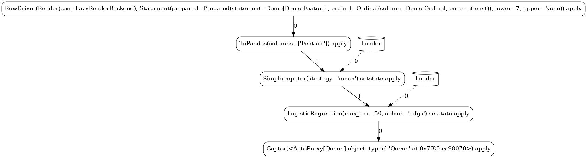
Starting with a minimal use case, this mini-pipeline contains just a single (stateful) operator - the RandomForestClassifier imported from the SKLearn library under the
operator auto-wrapping context which turns it transparently into a
true ForML operator.
To launch the pipeline, it is first bound to the Source
descriptor (declared previously in the common section) to dynamically assemble a virtual Artifact that
directly exposes a launcher instance. We select the
Graphviz runner (called visual in our
setup) and explicitly provide our shared Demo feed (since
that is not a platform-wide configured feed).
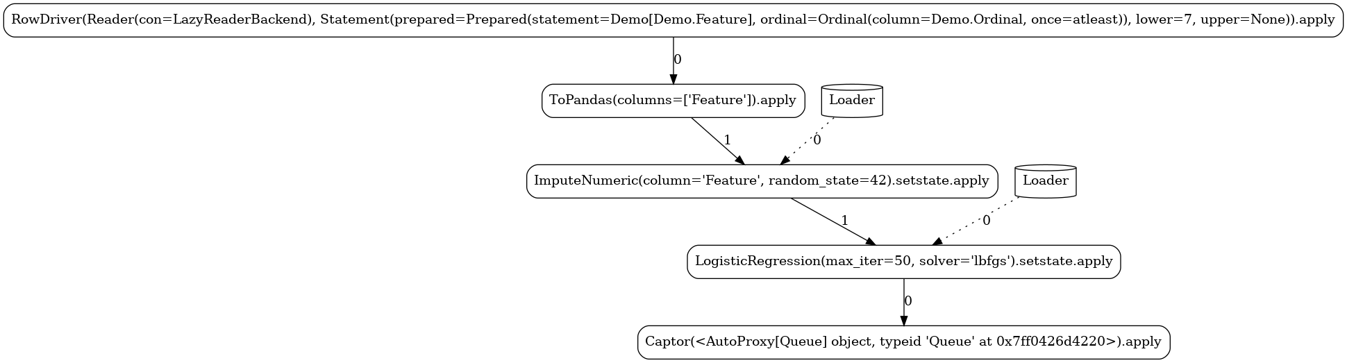
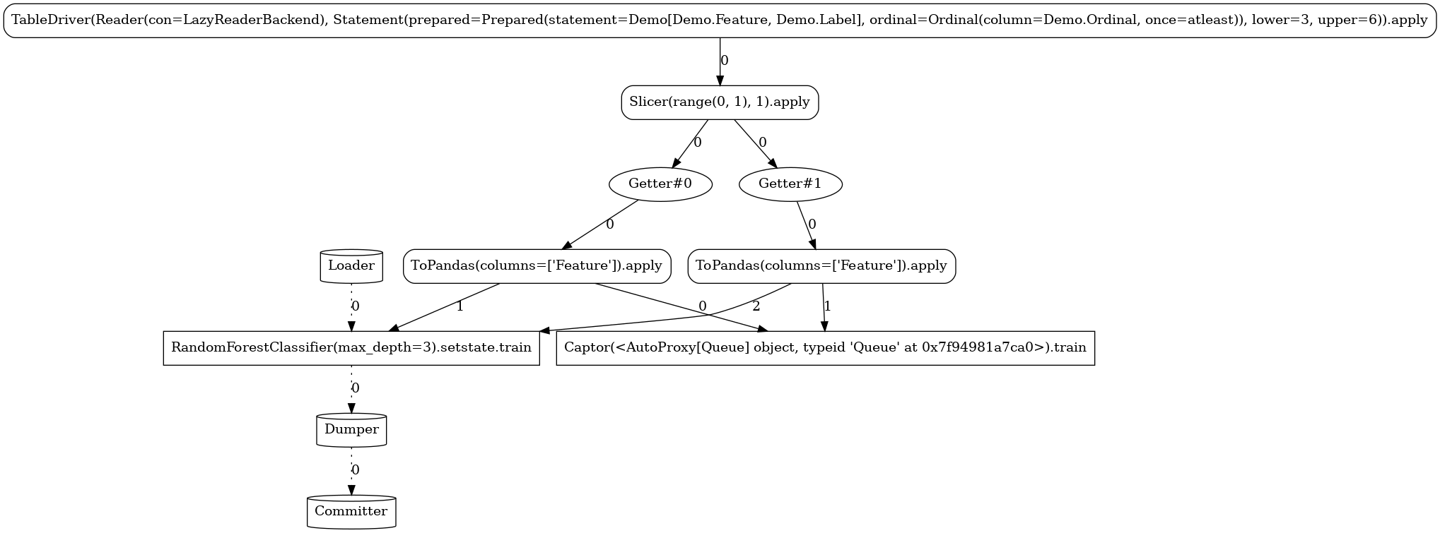
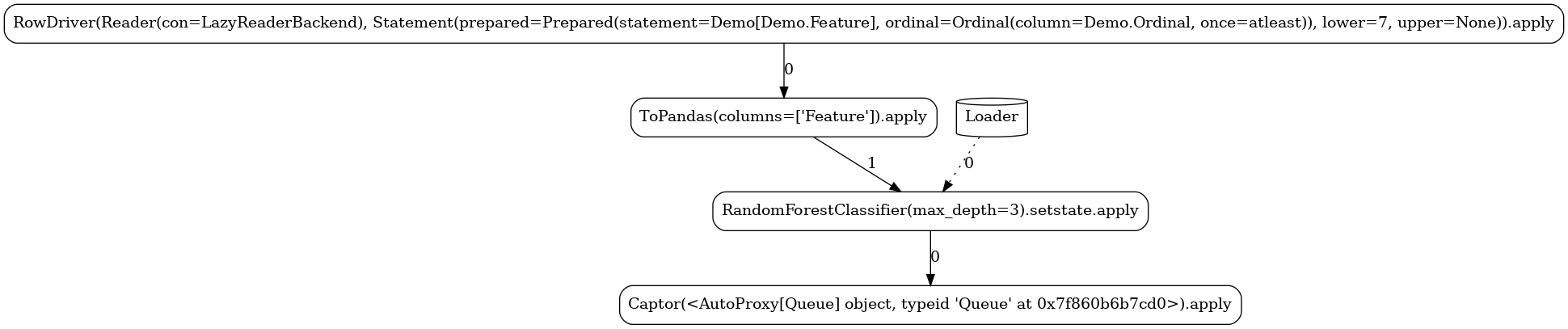
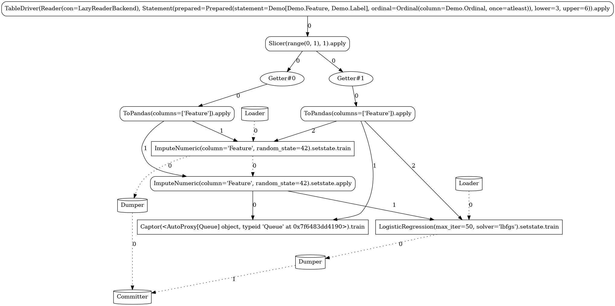
Below, you can see the different task graphs produced for each of the train versus apply
modes (note the ordinal lower/upper bounds specified when executing each
of the modes used as data filters with respect to the Data.Ordinal column). Apart from the
expected RandomForestClassifier node, the topology contains a number of additional tasks:
Source-related tasks (defined in our common section):the
feed readerthe positional label extractor (
Slicer)the explicitly defined stateless
ToPandastransformer
system nodes generated by the flow compiler (
Getter,Loader,Dumper,Comitter)the sink (
Captor) injected by the launcher
1 2 3 4 5 6 7 8 9 10 | |
LAUNCHER.train(3, 6)
LAUNCHER.apply(7)
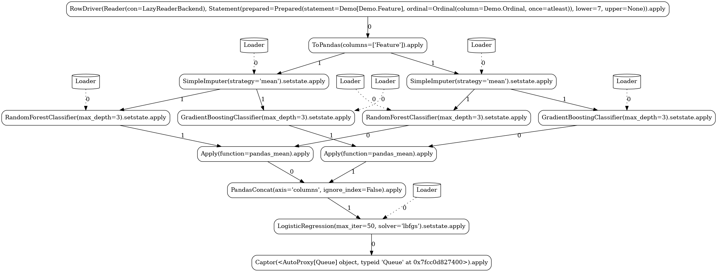
Simple
The next pipeline is demonstrating a true workflow expression of two (again stateful) operators participating in an operator composition:
1 2 3 4 5 6 7 8 9 10 11 | |
LAUNCHER.train(3, 6)
LAUNCHER.apply(7)
Ensemble
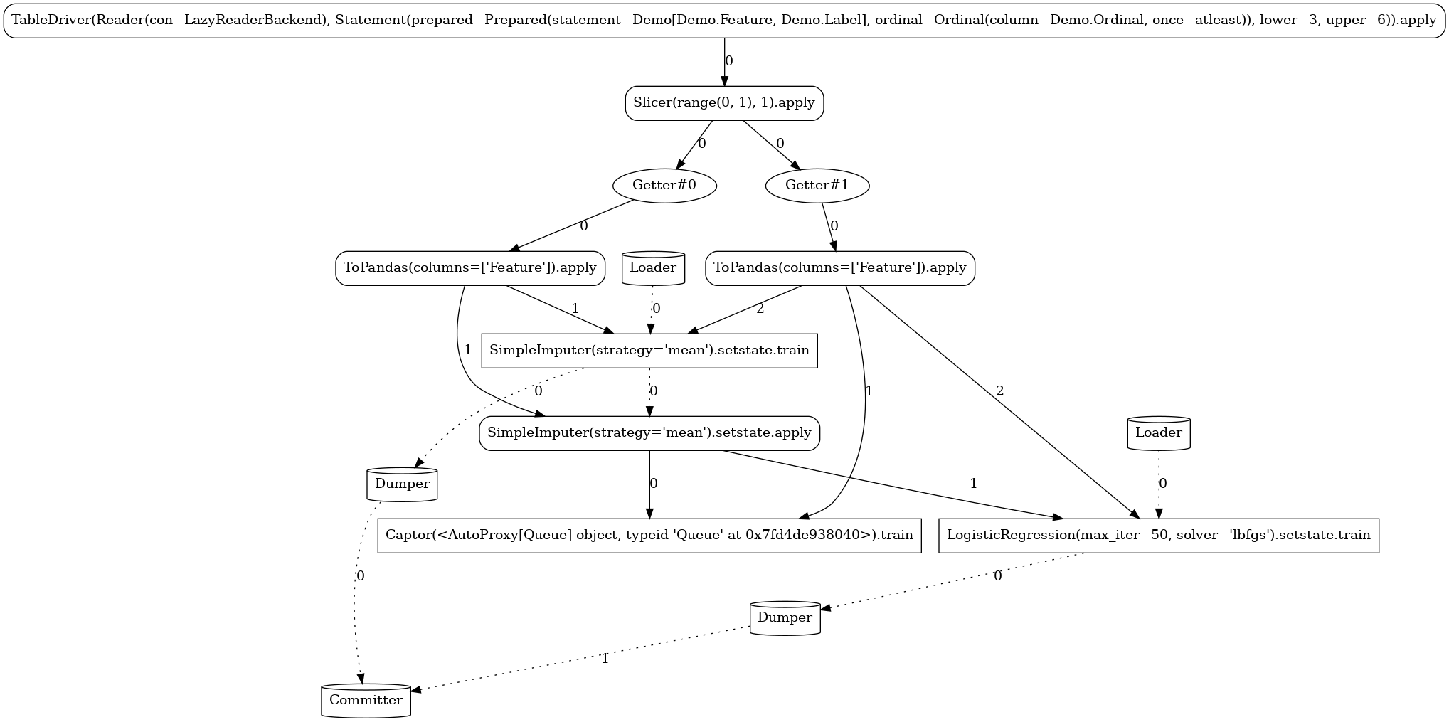
The ability to derive fairly involved workflows from simple expressions is demonstrated in the
following pipeline employing the model ensembling technique. For
readability, we use just two levels of folding (n_splits=2), the graph would be even more
complex with higher folding levels.
1 2 3 4 5 6 7 8 9 10 11 12 13 14 15 16 17 18 19 20 | |
LAUNCHER.train(3, 6)
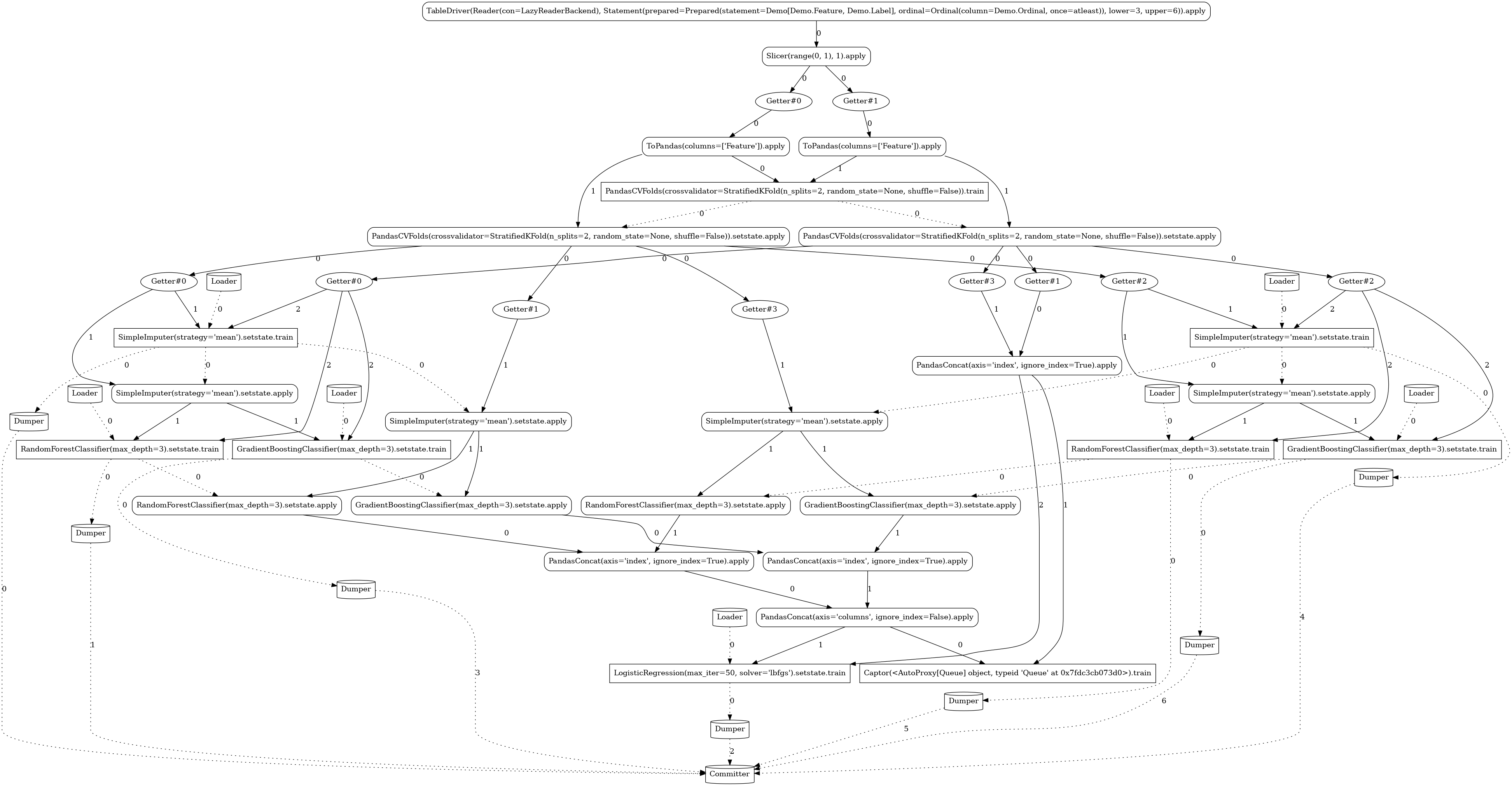
LAUNCHER.apply(7)
Complex
Going one step further, the following pipeline is again using the model ensembling technique, but
this time it defines a distinct transformation chain for each of the model branches
(OneHotEncoder for the RandomForestClassifier and Binarizer for BernoulliNB).
1 2 3 4 5 6 7 8 9 10 11 12 13 14 15 16 17 18 19 20 21 22 | |
LAUNCHER.train(3, 6)
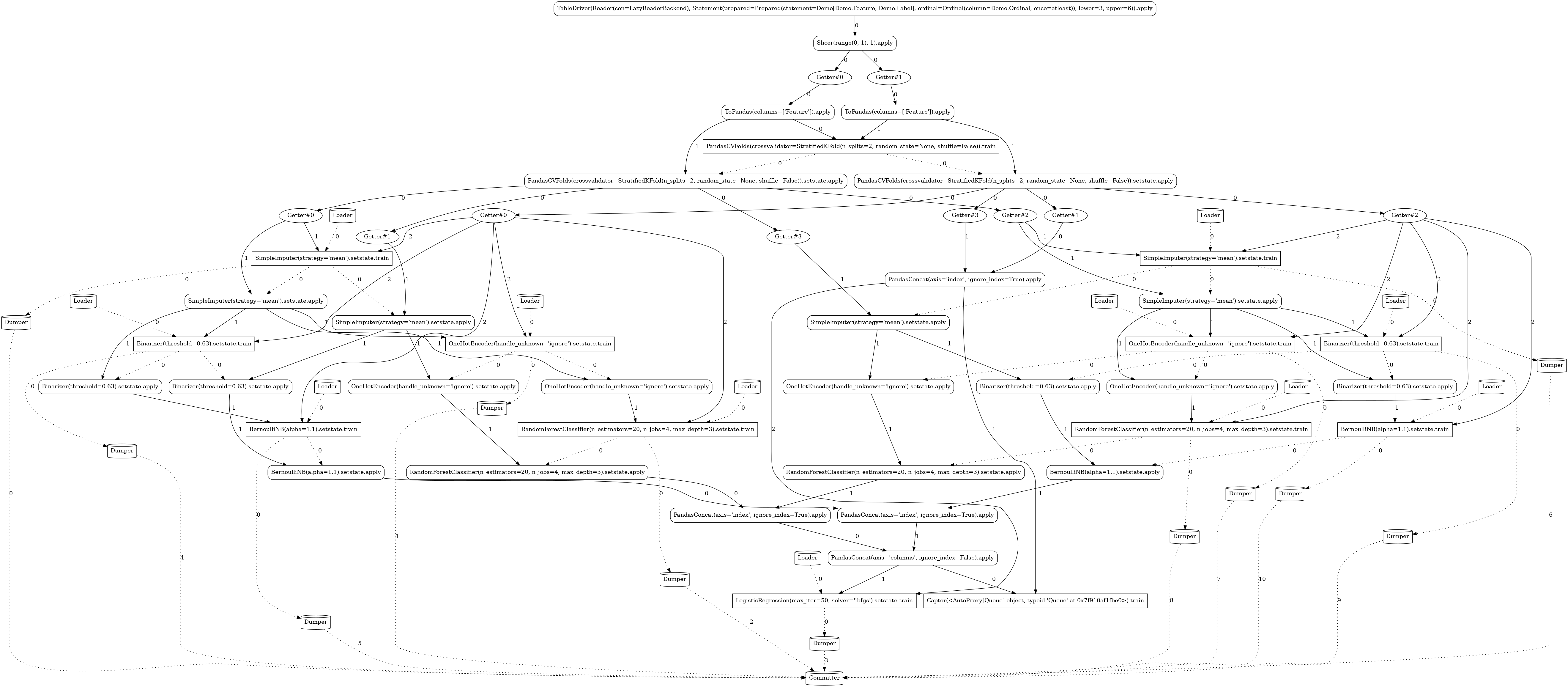
LAUNCHER.apply(7)

Custom
In this pipeline, we demonstrate the ability to define custom actors and
operators. We implement a simple stateful
mapper that at train mode persists the mean and standard
deviation of the observed column and at apply mode generates random integers within the given
mean±std range for any missing value.
1 2 3 4 5 6 7 8 9 10 11 12 13 14 15 16 17 18 19 20 21 22 23 24 25 26 27 28 29 30 31 32 33 34 35 36 37 38 39 40 41 42 | |
LAUNCHER.train(3, 6)
LAUNCHER.apply(7)